Monitor
The main function of the monitor is to monitor the changes of various variables during the network operation. In SPAIC, we have built-in two forms of monitors, namely StateMonitor and SpikeMonitor.
spaic.StateMonitor is designed to be used for tracking the state of Neurons , Connections and Nodes . spaic.SpikeMonitor is designed to be used for tracking the spike states and calculate the firing frequency.
self.mon_V = spaic.StateMonitor(self.layer1, 'V')
self.mon_O = spaic.StateMonitor(self.input, 'O')
self.spk_O = spaic.SpikeMonitor(self.layer1, 'O')
To initialize the monitor, we can specify the following parameters:
target – the object to be monitored. For StateMonitor, it can be any network module containing variables such as
NeuronGroupandConnection. For SpikeMonitor, it is generally a module with pulse distribution such asNeuronGroupandEncoder.var_name – the name of the variable that needs to be monitored, it needs to be a variable that the monitoring object has, such as the neuron’s membrane voltage ‘V’
index – the index value of the detection variable, for example, select a few neurons in a layer of neural clusters to record, you can use index=[1,3,4,…], the default is to record the entire variable
dt – the sampling interval of the monitor, defaults to the same as the simulation step size
get_grad – whether to record the gradient, True means the gradient is required, False means not required, the default is False
nbatch – whether you need to record the data of multiple batches, True will save the data of multiple runs, False will overwrite the data each time run, the default is False
Common functions to users in both StateMonitor and SpikeMonitor are:
monitor_on – Set the monitor to start the recording for current run. The monitor is set to be monitor_on by defualt.
monitor_on – Set the monitor to stop recording for current run.
clear – Clear all the recorded data in the monitor.
The difference between the two monitors is that StateMonitor has five property:
nbatch_times – logging the time step information of all batches, the shape structure of the data is (number of batches, number of time steps)
nbatch_values – logging the monitoring parameters of the target layer of all batches. The shape structure of the data is (batch, neuron, time step, sample in the batch)
times – logging the time step information of the current batch, the shape structure of the data is (number of time steps)
values – logging the monitoring variable of the target layer of the current batch. The shape structure of the data is (the number of samples in this batch, the number of neurons, the number of time steps)
tensor_values – logging the original tensor variable of the target layer of the current batch. The shape structure of the data is (the number of samples in this batch, the number of neurons, the number of time steps)
grad – logging the gradient of the target variable of the current batch, the shape of the data is the same as the shape of the values
And SpikeMonitor has another four property:
spk_index – logging the number of the neuron firing the current batch
spk_times – logging the time information of the current batch of pulses
time – logging information about the time step of the current batch
time_spk_rate – logging the instantaneous spike rate of the target layer for the current batch
spk_rate – logging the average spike rate of the target layer for the current batch
spk_count – logging each neuron’s spike count of the target layer for the current batch
Example code:
time_line = Net.mon_V.times # Take the time indices of layer1
value_line = Net.mon_V.values[0][0] # Take the voltage change records of the first neuron of layer 1 in this batch in the whole time window
input_line = Net.mon_O.values[0][0] # Take the spike records of the first neuron of input layer in this batch in the whole time window
# Since nbatch setted False when initialized, only have one batch
output_line_index = Net.spk_O.spk_index[0] + 1.2 # Take the spike index of this layer, since only have one neuron, add 1.2 to beautify the visualization appearance
output_line_time = Net.spk_O.spk_times[0] # Take the spike time index of this layer
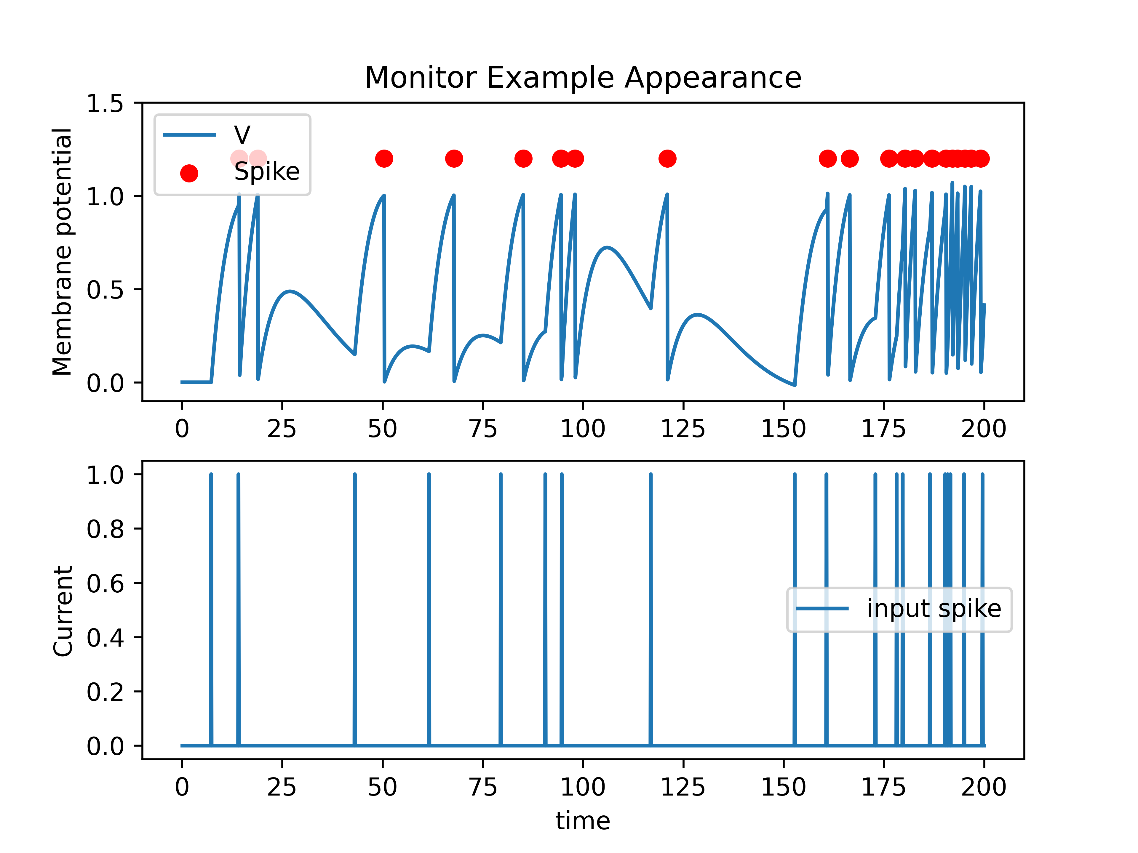
plt.subplot(2, 1, 1)
plt.title('Monitor Example Appearance')
plt.plot(time_line, value_line, label='V')
plt.scatter(output_line_time, output_line_index, s=40, c='r', label='Spike')
plt.ylabel("Membrane potential")
plt.ylim((-0.1, 1.5))
plt.legend()
plt.subplot(2, 1, 2)
plt.plot(time_line, input_line, label='input spike')
plt.xlabel("time")
plt.ylabel("Current")
plt.legend()
Result: